Module 7: Comparing RW only, the Census only, and RW + Census model

Outline

• Read in the outputs
• Compare Total Aboveground Biomass over time for each method (data-only estimates, TR only model, TR + census model)
• Compare Aboveground Biomass Increment over time for each method (data-only estimates, TR only model, TR + census model)
• Relating AGBI estimates to climate drivers

library(rstan)
library(dplyr)
library(reshape2)
library(ggplot2)
library(grid)
library(gridExtra)
library(tidyr)

1. Read in all of the outputs of each model

nchains = 1
iter = 500

##############################################
## 1. Load data
##############################################

# load built dataset
dat = readRDS('data/tree_data_HARVARD.RDS')

model_post_CENSUS <- readRDS("output/model_post_CENSUS_HARVARD.RDS")
model_post_RW <- readRDS("output/model_post_RW_HARVARD.RDS")
model_post_RW_CENSUS <- readRDS("output/model_post_RW_CENSUS_HARVARD.RDS")


fnames = paste0(c('model_post_RW',
                  'model_post_CENSUS',
                  'model_post_RW_CENSUS'), '_', 'HARVARD.RDS')
models = c('RW', 'Census', 'RW + Census')

nmodels = length(fnames)

# we only need "D" for diameter and we only need the iterations that we are planning to keep
post_d = list()
post_rw = list()
post_bt = list()
post_sx = list()
post_sxobs = list()
post_sdobs = list()
for (i in 1:length(fnames)) {
  fname_model = fnames[i]
  out = readRDS(paste0('output/', fname_model))

  # get all array slices for diameters
  variables = names(out[1,1,])
  allDs = grep('D\\[',variables)
  allRWs = grep('X\\[',variables)
  allBTs = grep('beta_t\\[',variables)
  allSX = grep('sig_x\\[',variables)
  allSXOBS = grep('sig_x_obs',variables)

  # we need to put into matrix for use in processing, some compile info from all chains
  out.temp.d = out[,,allDs]
  out.temp.rw = out[,,allRWs]
  out.temp.bt = out[,,allBTs]
  out.temp.sx = out[,,allSX]
  out.temp.sxobs = out[,,allSXOBS]
  # out.temp.sdobs = out[seq(dim(out)[1]-pool+1, dim(out)[1], pool/(keep/nchains)),,allSDOBS]

  # if(nchains>1){
  #   out = out.temp[,1,]
  #   out.rw = out.temp.rw[,1,]
  #   out.bt = out.temp.bt[,1,]
  #   out.sx = out.temp.sx[,1,]
  #
  #   for (j in 2:ncol(out.temp)){
  #     out = rbind(out, out.temp[,j,])
  #     out.rw = rbind(out.rw, out.temp.rw[,j,])
  #     out.sx = rbind(out.rw, out.temp.sx[,j,])
  #   }
  #   post[[i]] = out
  #   post_rw[[i]] = out.rw
  # } else {
  post_d[[i]] = out.temp.d
  post_rw[[i]] = out.temp.rw
  post_bt[[i]] = out.temp.bt
  post_sx[[i]] = out.temp.sx
  post_sx[[i]] = out.temp.sx
  post_sxobs[[i]] = out.temp.sxobs
  # }

  # if (models[i] == 'Census'){
  #   allSDOBS = grep('sig_d_obs',variables)
  #   out.temp.sdobs = out[,,allSDOBS]
  #   # if(nchains>1){
  #   #   out.sdobs = out.temp.sdobs[,1,]
  #   #   for (j in 2:ncol(out.temp.sdobs)){
  #   #     out.sdobs = rbind(out.sdobs, out.temp.sdobs[,j,])
  #   #   }
  #   # } else {
  #     out.sdobs = out.temp.sdobs
  #   # }
  #   post_sdobs_C = out.sdobs
  #   sigma_d_obs_C = median(post_sdobs_C)
  # }
  #
  # if (models[i] == 'RW + Census'){
  #   allSDOBS = grep('sig_d_obs',variables)
  #   out.temp.sdobs = out[,,allSDOBS]
  #   if(nchains>1){
  #     out.sdobs = out.temp.sdobs[,1,]
  #     for (j in 2:ncol(out.temp.sdobs)){
  #       out.sdobs = rbind(out.sdobs, out.temp.sdobs[,j,])
  #     }
  #   } else {
  #     out.sdobs = out.temp.sdobs
  #   }
  #   post_sdobs_RWC = out.sdobs
  #   sigma_d_obs_RWC = median(post_sdobs_RWC)
  # }

}

#
# # load built data for site
# dat = readRDS(file.path(site_dir,'runs',paste0(mvers,'_',dvers),'input',paste0('tree_data_', site ,'_STAN_',mvers,'_', dvers, '.RDS')))
N_years = dat$N_years
N_Tr = dat$N_Tr
N_taxa = dat$N_taxa
X2Tr = dat$X2Tr
X2year = dat$X2year
Tr = dat$Tr %>% arrange(stat_id)
taxon = Tr$taxon
plot = Tr$plot
years = dat$years
year_lo = min(years)
year_hi = max(years)
# sig_d_obs = dat$sig_d_obs
pdbh = exp(dat$logTr)
#
list2env(dat, envir = globalenv())

<environment: R_GlobalEnv>

N_C = dat$N_C
X2C = dat$X2C
X2year_C = dat$X2year_C

allTrees = dat$allTrees %>% arrange(stat_id)
taxon_C = allTrees$taxon
plot_C = allTrees$plot
distance = allTrees$distance

tree <- 1
# pdf('figures/tree_growth_model_ALL.pdf', width=10, height=6)
# for (tree in 1:N_C){

  print(tree)

[1] 1

  in.RW = tree %in% X2Tr

  if (in.RW){
    inds = which(X2Tr == tree)
    yrinds = X2year[inds]

    dbh_iter = t(post_d[[1]][,inds])
    dbh_iter = data.frame(dbh_iter)
    dbh_iter = data.frame(year=years[yrinds], dbh_iter)

    dbh_mean = apply(dbh_iter[,2:ncol(dbh_iter)], 1, mean, na.rm=TRUE)
    dbh_quant = t(apply(dbh_iter[,2:ncol(dbh_iter)], 1,
                        function(x) quantile(x, c(0.025, 0.5, 0.975), na.rm=TRUE)))

    dbh_tree = data.frame(d_mean = dbh_mean,
                          d_median = dbh_quant[,2],
                          d_lo = dbh_quant[,1],
                          d_hi = dbh_quant[,3],
                          year = years[yrinds],
                          model = 'RW')

  }

  # determine which estimates correspond to this tree
  inds_C = which(X2Tr_C == tree)
  yrinds_C = X2year_C[inds_C]

  # C
  dbh_iter_C = t(post_d[[2]][,inds_C])
  dbh_iter_C = data.frame(dbh_iter_C)
  dbh_iter_C = data.frame(year=years[yrinds_C], dbh_iter_C)

  dbh_mean_C = apply(dbh_iter_C[,2:ncol(dbh_iter_C)], 1, mean, na.rm=TRUE)
  dbh_quant_C = t(apply(dbh_iter_C[,2:ncol(dbh_iter_C)], 1,
                        function(x) quantile(x, c(0.025, 0.5, 0.975), na.rm=TRUE)))

  dbh_tree_C = data.frame(d_mean = dbh_mean_C,
                          d_median = dbh_quant_C[,2],
                          d_lo = dbh_quant_C[,1],
                          d_hi = dbh_quant_C[,3],
                          year = years[yrinds_C],
                          model = 'Census')

  # RWC
  dbh_iter_RWC = t(post_d[[3]][,inds_C])
  dbh_iter_RWC = data.frame(dbh_iter_RWC)
  dbh_iter_RWC = data.frame(year=years[yrinds_C], dbh_iter_RWC)

  dbh_mean_RWC = apply(dbh_iter_RWC[,2:ncol(dbh_iter_RWC)], 1, mean, na.rm=TRUE)
  dbh_quant_RWC = t(apply(dbh_iter_RWC[,2:ncol(dbh_iter_RWC)], 1,
                          function(x) quantile(x, c(0.025, 0.5, 0.975), na.rm=TRUE)))

  dbh_tree_RWC = data.frame(d_mean = dbh_mean_RWC,
                            d_median = dbh_quant_RWC[,2],
                            d_lo = dbh_quant_RWC[,1],
                            d_hi = dbh_quant_RWC[,3],
                            year = years[yrinds_C],
                            model = 'RW + Census')

  if (in.RW){
    dbh_tree = rbind(dbh_tree,
                     dbh_tree_C,
                     dbh_tree_RWC)
  } else {
    dbh_tree = dbh_tree_C
  }

  idx_d_obs_C = which(Dobs$stat_id == tree)

  dbh_obs_C = data.frame(d_obs = Dobs$dbh[idx_d_obs_C],
                         year = years[Dobs$year[idx_d_obs_C]])

  stem_id = Dobs$ID[idx_d_obs_C][1]

  if (in.RW){
    idx_d_obs = which(Tr$stat_id == tree)

    dbh_obs = data.frame(d_obs = Tr$dbh[idx_d_obs],
                         year = years[Tr$year[idx_d_obs]])

  } else {
    dbh_obs = data.frame(d_obs = numeric(0),
                         year = numeric(0))
  }

  # Create a text
  grob = grobTree(textGrob(paste0('Tree ', tree, '; Stem ID ', stem_id, '; Species ', taxon[tree] ), x=0.05,  y=0.9, hjust=0,
                           gp=gpar(col="black", fontsize=22)))

  p1 = ggplot() +
    geom_ribbon(data=dbh_tree, aes(x=year, ymin=d_lo, ymax=d_hi, fill=model), alpha=0.5) +
    geom_line(data=dbh_tree, aes(x=year, y=d_median, colour=model)) +
    geom_point(data=dbh_obs, aes(x=year, y=d_obs), size=2) +
    geom_point(data=dbh_obs_C, aes(x=year, y=d_obs), size=2, shape=1) +
    xlab('year') +
    ylab('dbh (cm)') +
    xlim(c(year_lo, year_hi)) +
    theme_bw(16)  +
    annotation_custom(grob)

  print(p1)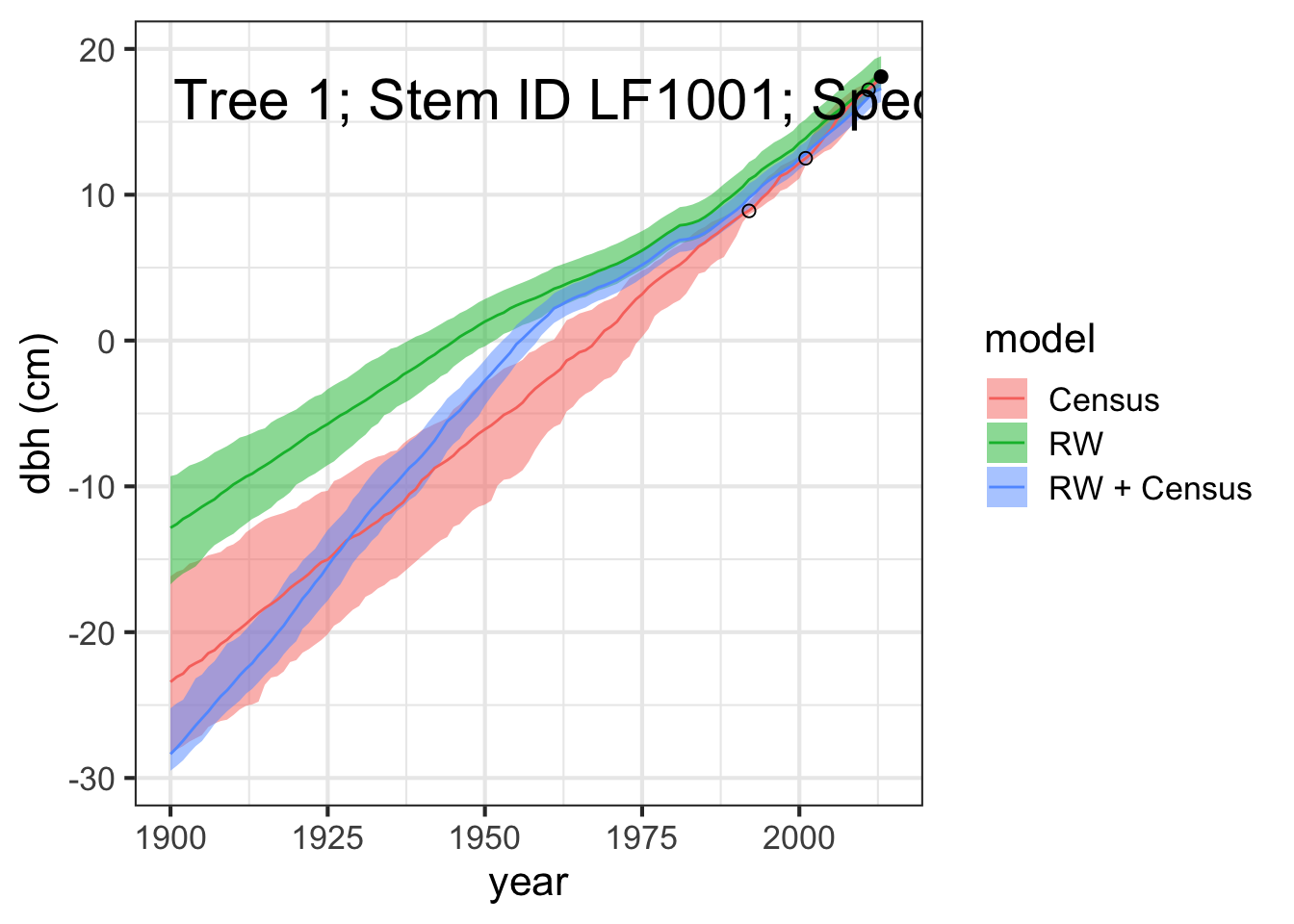

  if (in.RW){
    inds = which(X2Tr == tree)
    yrinds = X2year[inds]

    rw_iter = t(post_rw[[1]][,inds])
    rw_iter = data.frame(rw_iter)
    rw_iter = data.frame(year=years[yrinds], rw_iter)

    rw_mean = apply(rw_iter[,2:ncol(rw_iter)], 1, mean, na.rm=TRUE)
    rw_quant = t(apply(rw_iter[,2:ncol(rw_iter)], 1,
                       function(x) quantile(x, c(0.025, 0.5, 0.975), na.rm=TRUE)))

    rw_tree = data.frame(x_mean = rw_mean,
                         x_median = rw_quant[,2],
                         x_lo = rw_quant[,1],
                         x_hi = rw_quant[,3],
                         year = years[yrinds],
                         model = 'RW')
  }


  inds_C = which(X2Tr_C == tree)
  yrinds_C = X2year_C[inds_C]

  rw_iter_C = t(post_rw[[2]][,inds_C])
  rw_iter_C = data.frame(rw_iter_C)
  rw_iter_C = data.frame(year=years[yrinds_C], rw_iter_C)

  rw_mean_C = apply(rw_iter_C[,2:ncol(rw_iter_C)], 1, mean, na.rm=TRUE)
  rw_quant_C = t(apply(rw_iter_C[,2:ncol(rw_iter_C)], 1,
                       function(x) quantile(x, c(0.025, 0.5, 0.975), na.rm=TRUE)))

  rw_tree_C = data.frame(x_mean = rw_mean_C,
                         x_median = rw_quant_C[,2],
                         x_lo = rw_quant_C[,1],
                         x_hi = rw_quant_C[,3],
                         year = years[yrinds_C],
                         model = 'Census')

  rw_iter_RWC = t(post_rw[[3]][,inds_C])
  rw_iter_RWC = data.frame(rw_iter_RWC)
  rw_iter_RWC = data.frame(year=years[yrinds_C], rw_iter_RWC)

  rw_mean_RWC = apply(rw_iter_RWC[,2:ncol(rw_iter_RWC)], 1, mean, na.rm=TRUE)
  rw_quant_RWC = t(apply(rw_iter_RWC[,2:ncol(rw_iter_RWC)], 1,
                         function(x) quantile(x, c(0.025, 0.5, 0.975), na.rm=TRUE)))

  rw_tree_RWC = data.frame(x_mean = rw_mean_RWC,
                           x_median = rw_quant_RWC[,2],
                           x_lo = rw_quant_RWC[,1],
                           x_hi = rw_quant_RWC[,3],
                           year = years[yrinds_C],
                           model = 'RW + Census')


  if (in.RW){
    rw_tree = rbind(rw_tree,
                    rw_tree_C,
                    rw_tree_RWC)
  } else {
    rw_tree = rw_tree_C
  }


  if (in.RW){
    idx_rw_obs = which(Xobs$stat_id == tree)

    rw_obs = data.frame(x_obs = Xobs$incr[idx_rw_obs],
                        year = years[Xobs$year[idx_rw_obs]])
  } else {
    rw_obs = data.frame(x_obs = numeric(0),
                        year = numeric(0))
  }

  # Create a text
  grob <- grobTree(textGrob(paste0('Tree ', tree, '; Stem ID ', stem_id, '; Species ', taxon[tree] ), x=0.05,  y=0.9, hjust=0,
                            gp=gpar(col="black", fontsize=22)))

  p2 = ggplot() +
    # geom_line(data=dbh_tree, aes(x=year, y=d_mean)) +
    # geom_ribbon(data=rw_tree, aes(x=year, ymin=x_lo, ymax=x_hi), fill='lightgrey') +
    geom_ribbon(data=rw_tree, aes(x=year, ymin=x_lo, ymax=x_hi, fill=model), alpha=0.5) +
    geom_line(data=rw_tree, aes(x=year, y=x_median, colour=model)) +
    geom_point(data=rw_obs, aes(x=year, y=x_obs), size=2, alpha=0.4) +
    # geom_dog(data=rw_obs, aes(x=year, y=x_obs, dog='glasses'), size=2) +
    # ylim(c(0,500)) +
    xlab('year') +
    ylab('rw (mm)') +
    xlim(c(year_lo, year_hi)) +
    theme_bw(16)  #+
  # ggtitle(paste0('Tree ', i)) +
  # annotation_custom(grob)

  # print(p2)

  grid.arrange(p1, p2, nrow = 2)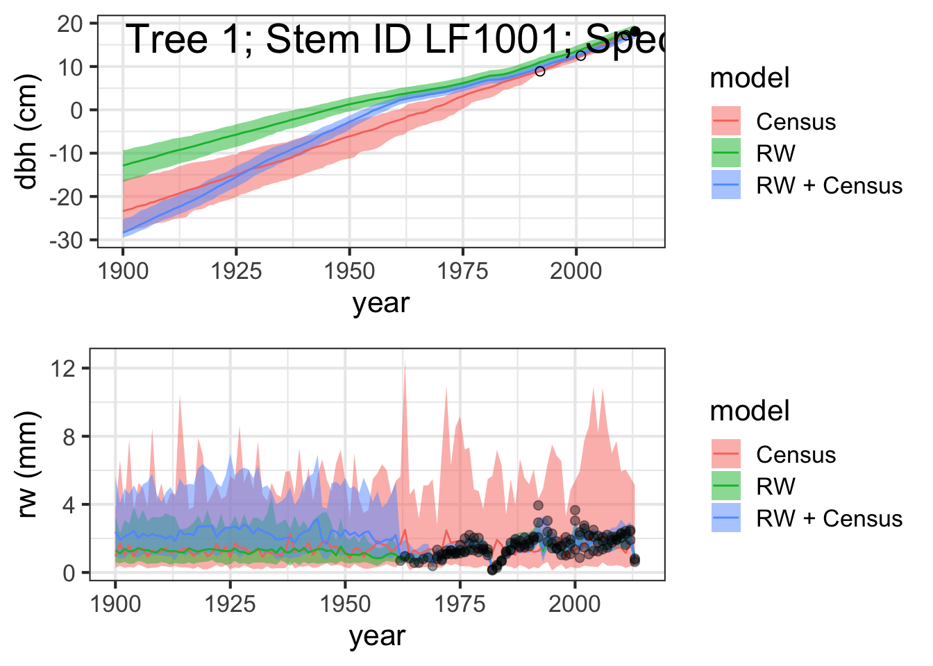

#}

2. Read in estimated biomass from all 3 models

abi_site_CENSUS <- readRDS( "summary/abi_site_summary_CENSUS.RDS")
agb_site_CENSUS <- readRDS("summary/agb_site_summary_CENSUS.RDS")

abi_taxon_CENSUS <- readRDS( "summary/abi_taxon_summary_CENSUS.RDS")
agb_taxon_CENSUS <- readRDS("summary/agb_taxon_summary_CENSUS.RDS")

abi_site_TR <- readRDS( "summary/abi_site_summary_TR.RDS")
agb_site_TR <- readRDS("summary/agb_site_summary_TR.RDS")

abi_taxon_TR <- readRDS( "summary/abi_taxon_summary_TR.RDS")
agb_taxon_TR <- readRDS("summary/agb_taxon_summary_TR.RDS")


abi_site_TR_CENSUS <- readRDS( "summary/abi_site_summary_TR_CENSUS.RDS")
agb_site_TR_CENSUS <- readRDS("summary/agb_site_summary_TR_CENSUS.RDS")

abi_taxon_TR_CENSUS <- readRDS( "summary/abi_taxon_summary_TR_CENSUS.RDS")
agb_taxon_TR_CENSUS <- readRDS("summary/agb_taxon_summary_TR_CENSUS.RDS")

3. Plot up total AGB and AGBI over time for each method

Taxon-level Aboveground Biomass (AGB) and Aboveground Biomass Increment (AGBI)

agb_site_summary <- rbind(agb_site_TR, agb_site_CENSUS, agb_site_TR_CENSUS)
abi_site_summary <- rbind(abi_site_TR, abi_site_CENSUS, abi_site_TR_CENSUS)

agb_taxon_summary <- rbind(agb_taxon_TR, agb_taxon_CENSUS, agb_taxon_TR_CENSUS)
abi_taxon_summary <- rbind(abi_taxon_TR, abi_taxon_CENSUS, abi_taxon_TR_CENSUS)

ggplot(data = agb_taxon_summary)+
  geom_ribbon(aes(x=year, ymin=AGB.lo, ymax=AGB.hi, colour=model, fill=model), alpha=0.4, linetype=2) +
  geom_line(aes(x = year, y = AGB.mean, color = model))+
  facet_grid(taxon~., scales='free_y') +
  theme_light(18) +
  ylab('Taxa Aboveground Biomass (mg/ha)')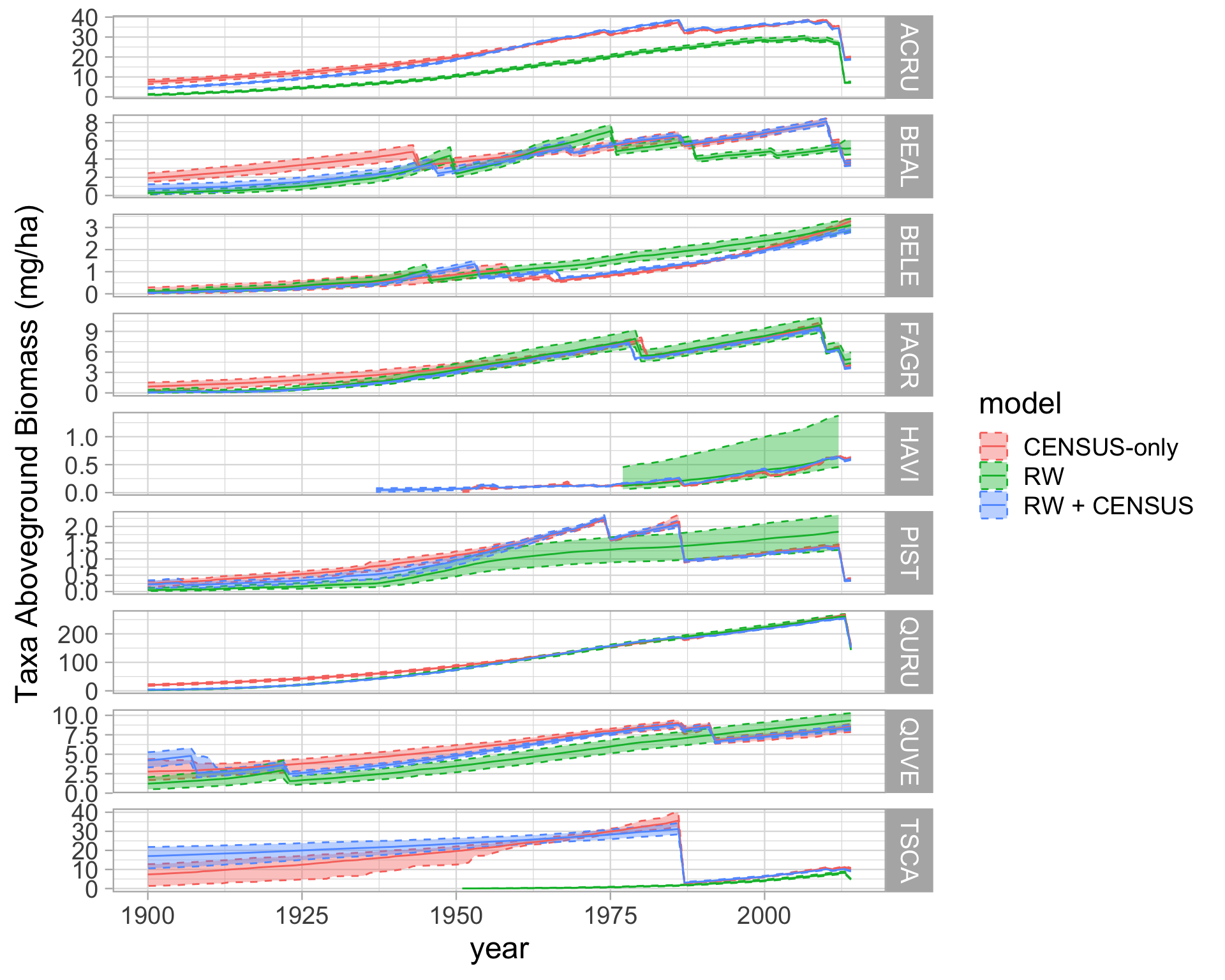

ggplot(data = abi_taxon_summary)+
  geom_ribbon(aes(x=year, ymin=ABI.lo, ymax=ABI.hi, colour=model, fill=model), alpha=0.4, linetype=2) +
  geom_line(aes(x = year, y = ABI.mean, color = model))+
  facet_grid(taxon~., scales='free_y') +
  theme_light(18) +
  ylab('Taxa biomass increment (mg/ha)')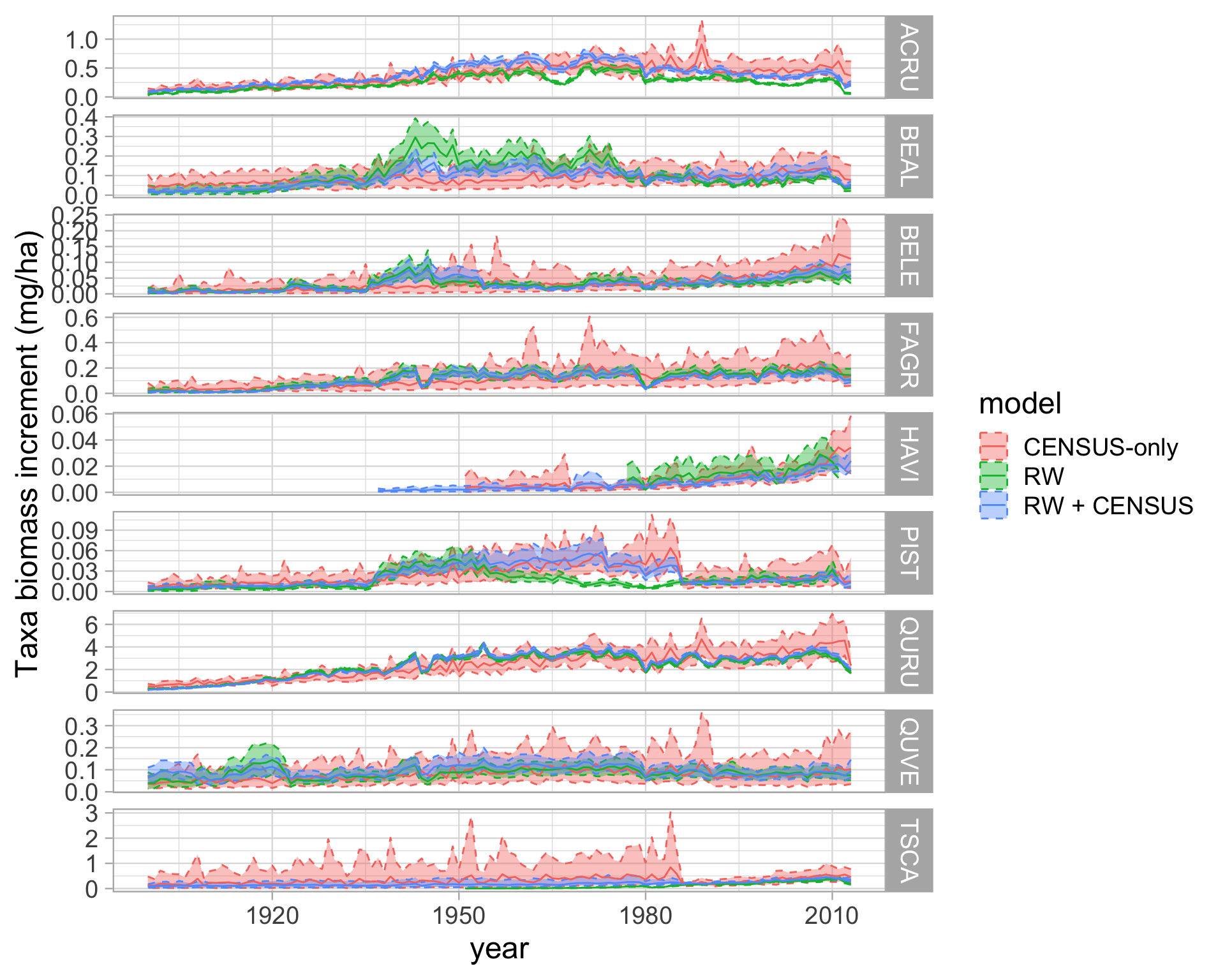

Stand-level Biomass and Biomass increment

Plot up stand-scale AGB over time for each method

ggplot(data = agb_site_summary)+
  geom_ribbon(aes(x=year, ymin=ab025, ymax=ab975, fill = model), alpha=0.4, linetype=2) +
  geom_line(aes(x = year, y = abmean, color = model))+
  #facet_grid(model~., scales='free_y') +
  theme_light(18) +
  ylab('biomass (mg/ha)')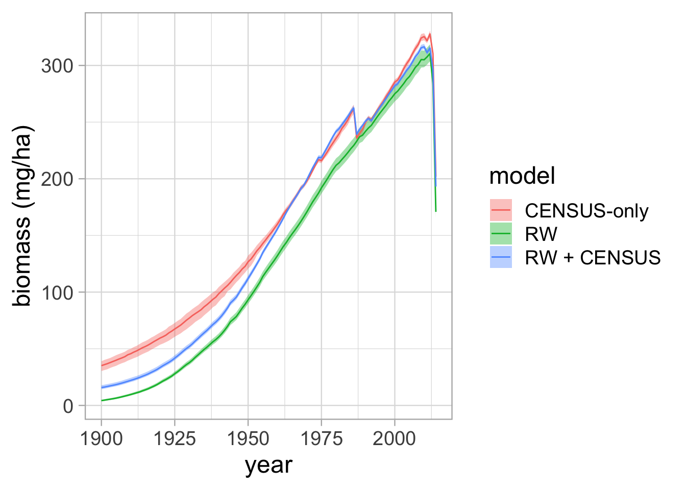

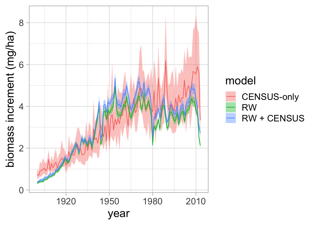
Plot up stand-scale AGBI over time for each method

ggplot(data = abi_site_summary)+
  geom_ribbon(aes(x=year, ymin=abi025, ymax=abi975, fill = model), alpha=0.4, linetype=2) +
  geom_line(aes(x = year, y = abimean, color = model))+
  #facet_grid(model~., scales='free_y') +
  theme_light(18) +
  ylab('biomass increment (mg/ha)')