Module 2: Data: Tree Ring and Census Data

Load packages to be used

packages <- c("ggplot2", "tidyverse", "rstan", "dplR", "reshape2")
install.packages(setdiff(packages, rownames(installed.packages())))  

library(ggplot2)
library(tidyverse)
library(rstan)

Notes on running this tutorial

Boxes like this one above contain R code to run this analysis. Clicking the arrow character in the upper right corner of the box will expand or collapse the contents of the box.

Module 2 Objectives

• visualize Harvard Forest Tree Ring and Forest Census Data

Tree Ring Data

Harvard Forest tree ring data

There are two foundational datasets used in the processing of these biomass estimates. The first is a tree ring dataset collected by the Harvard Forest Research Area in 2012. Three 20m plots were measured following a double-nested design. The following species were included in the final ring width dataset:

• ACRU = red maple (Acer rubrum)
• BEAL = yellow birch (Betula alleghaniensis)
• BELE = sweet birch (Betula lenta)
• FAGR = American beech (Fagus grandifolia)
• HAVI = Witch hazel (Hamamelis virginiana)
• PIST = Eastern white pine (Pinus strobus)
• QURU = Northern red oak (Quercus rubra)
• QUVE = Black oak (Quercus velutina)
• TSCA = Eastern hemlock (Tsuga canadensis)

Harvard forest tree ring data samples were collected

Citation on tree ring dataset: Dye, A. Barker Plotkin, D. Bishop, N. Pederson, B. Poulter, and A. Hessl. Comparing tree-ring and permanent plot estimates of aboveground net primary production in three eastern us forests. Ecosphere, 7(9), 2016.

• We downloaded the raw data for Harvard Forest Tree ring data for you
• Visualize the pre-formatted HF tree ring data below

# code to plot the tree ring data, by species
HARV <- readRDS("data/tree_data_HARVARD.RDS")
taxon.conversion <- readRDS("data/taxon_conversion.RDS")

# Xobs contains the increment data for all the cored trees
head(HARV$Xobs)

      id year incr plot stat_id taxon
1 LF1001   63 0.69    1       1  TSCA
2 LF1001   64 0.95    1       1  TSCA
3 LF1001   65 0.83    1       1  TSCA
4 LF1001   66 0.57    1       1  TSCA
5 LF1001   67 0.58    1       1  TSCA
6 LF1001   68 0.79    1       1  TSCA

# Tr contains the diameter at the closest measured year for each cored tree
head(HARV$Tr)

  stat_id plot     id year  dbh distance taxon
1       1    1 LF1001  114 18.1      7.6  TSCA
2       2    1 LF1002  114 66.0      7.2  QURU
3       3    1 LF1003  113 22.3      7.5  ACRU
4       4    1 LF1004  113 30.4     10.6  ACRU
5       5    1 LF1005  113 15.6      9.7  ACRU
6       6    1 LF1007  113 30.0     11.9  BEAL

# combine the tree ring data with their diameters
Tree.ring <- HARV$Xobs %>% left_join(., HARV$Tr)

# get the calendar years
year.df <- data.frame(year = max(Tree.ring$year):1, 
                      cal.year = 2012:(2013 - max(Tree.ring$year)))
Tree.ring <- Tree.ring %>% left_join(., year.df)

# make a timeseries plot of all the tree ring increments
ggplot(data = Tree.ring)+geom_line(aes(x = cal.year, y = incr, group = id, color = taxon), alpha = 0.5)+facet_wrap(~taxon)+ylab("Increment (mm)")+xlab("Year")+theme_bw()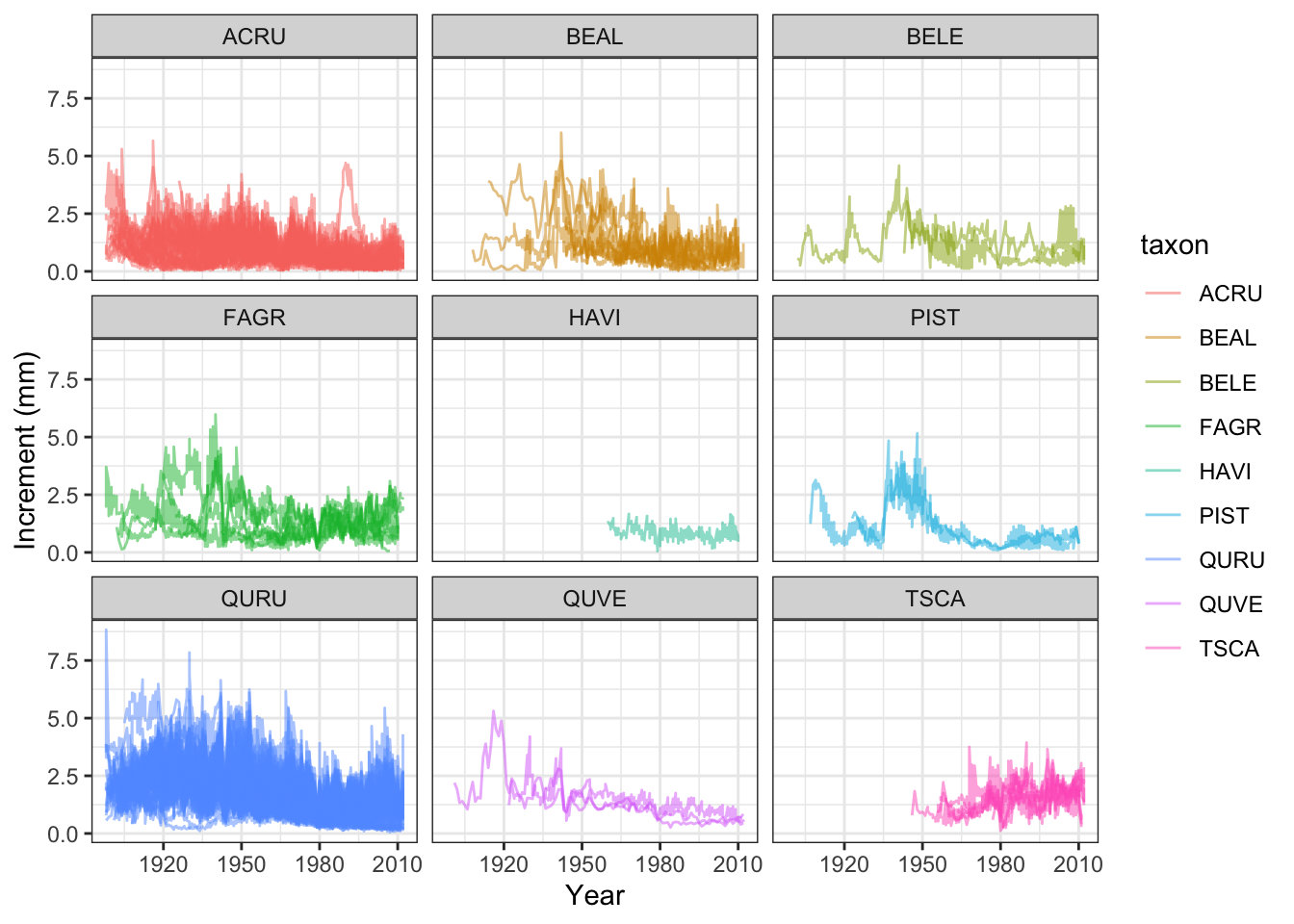

# plot the diameter measurements for the cored trees
ggplot(data = Tree.ring)+geom_point(aes(x = cal.year, y = dbh, group = id, color = taxon), alpha = 0.5)+facet_wrap(~taxon)+ylab("Increment (mm)")+xlab("Year")+theme_bw()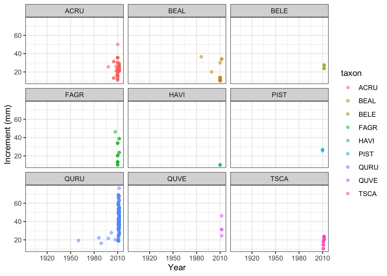

Harvard Forest Census Data

The second dataset for this site includes the census data measured for the Lyford Plots, which is available on the Harvard Forest data archive website. Censuses were conducted in 1962, 1969, 1975, 1987-1991, 2001, and 2011 and mapped all trees with DBH greater than 5 cm. in a mapped area covering 2.88 ha. The three ring-width plots include only a fraction of this area, and, therefore, we determined which census trees were located within the plot areas and considered only those trees for the model.

# code to plot census data, by species
# - ACRU = red maple (Acer rubrum) 
# - BEAL = yellow birch (Betula alleghaniensis) 
# - BELE = sweet birch (Betula lenta)
# - FAGR = American beech (Fagus grandifolia) 
# - HAVI = Witch hazel (Hamamelis virginiana) 
# - PIST = Eastern white pine (Pinus strobus)
# - QURU = Northern red oak (Quercus rubra) 
# - QUVE = Black oak (Quercus velutina)
# - TSCA = Eastern hemlock (Tsuga canadensis)


# set up the lat-long information:
HARV.ll <- data.frame(site = c("LF1", "LF2", "LF3"), 
                      lat = c(42.53065, 42.53128, 42.53008), 
                      lon = c(-72.18346, -72.18271, -72.18246))

Census <- HARV$Dobs %>% left_join(., year.df) %>% 
  rename("taxon" = "species")%>%
  left_join(., taxon.conversion) %>%# combine with taxon-infomation
  left_join(., HARV.ll) # combine with lat-long information

ggplot(data = Census)+geom_point(aes(x = cal.year, y = dbh, group = ID, color = `Scientific Name`, shape = finalCond), alpha = 0.5)+ geom_line(aes(x = cal.year, y = dbh, group = ID, color = `Scientific Name`)) + facet_wrap(~site, ncol = 3)+ylab("DBH (cm)")+xlab("Year")+theme_bw()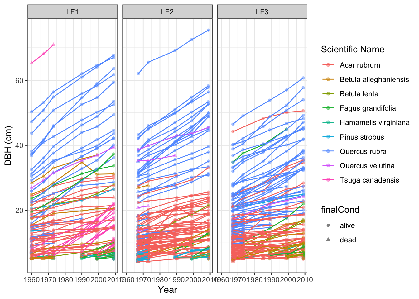

Note that for two of the plots at Harvard Forest, the census was split over mutiple years (1985-1990), creating an “inventory year” variable will allow us to compare tree estimates over each census

ggplot(data = Census)+
  geom_bar(aes(x = cal.year, fill = `Scientific Name`), stat = "count")+  facet_wrap(~site, ncol = 3)+xlab("Year")+theme_bw()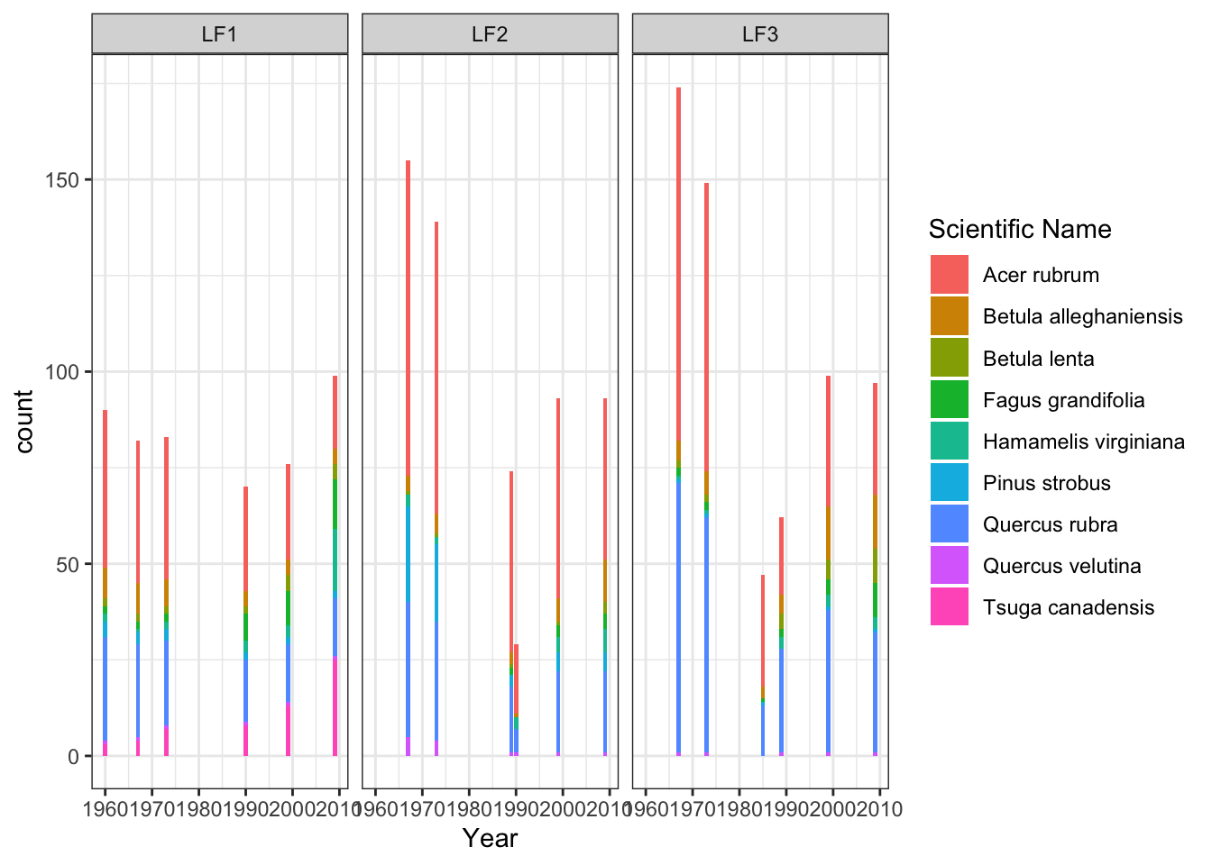

#Census dates: 1962, 1969, 1975, 1985-1991, 2001, and 2011
Census <- Census %>% 
  mutate(INV.YEAR = ifelse(cal.year >= 1985 & cal.year <= 1991, 1990, cal.year))

ggplot(data = Census)+
  geom_bar(aes(x = INV.YEAR, fill = `Scientific Name`), stat = "count")+  facet_wrap(~site, ncol = 3)+xlab("Year")+theme_bw()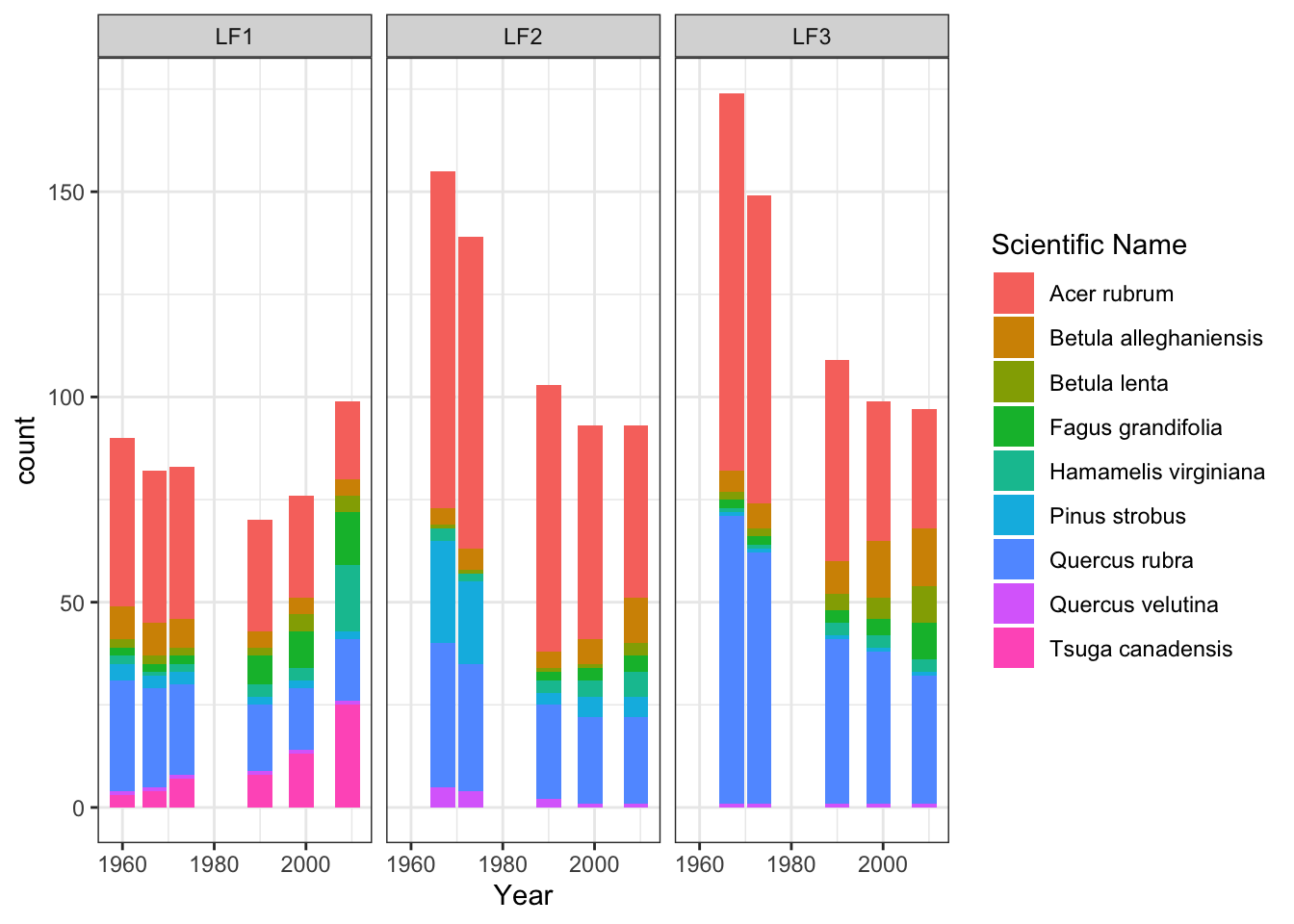

In the next module:

We will learn how to back-calculate tree diameters from tree ring data and how to scale tree diameter measurements up to tree-level biomass and carbon

Additional information:

Some tree census data sources of regional interest include:

- ForestGEO forest census plots (Cameroon, Congo, Gabon, Kenya, Nigeria) -